How High is a Coaxial Cable’s Max Frequency?

Struggling with signal loss at high frequencies? You've picked the perfect coaxial cable, but your system still isn't performing as expected, costing you time and project delays.

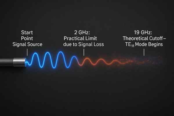
A coaxial cable's maximum frequency isn't a single number. It's limited by its cutoff frequency, where higher-order modes like \(TE_{11}\) begin to propagate. For a standard RG58 cable, this theoretical limit is around 19 GHz, but practical use is limited by excessive signal loss to well below 2 GHz.

Understanding this limit is just the beginning. The real challenge is that a cable's performance depends on many factors, not just one number on a datasheet. In my years as a hardware engineer, I've seen countless projects get delayed because of issues that seemed to come from nowhere, but were actually rooted in a misunderstanding of how RF cables work. To truly master high-frequency design, you need to look deeper into how these cables work and what really limits them. Let's break it down.

---

How is Coaxial Cable Attenuation Specified and Calculated?

Is your signal strength dropping off more than you predicted? Calculating cable loss seems straightforward, but real-world results often don't match, causing frustrating redesigns and performance issues.

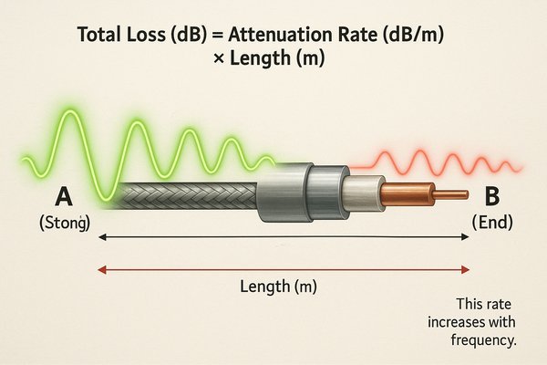
Coaxial cable attenuation is specified in decibels per unit length (e.g., dB/100m or dB/100ft) at specific frequencies. To calculate the total loss for a given length and frequency, you use the formula: \(\text{Total Loss (dB)} = \text{Attenuation Rate (dB/m)} \times \text{Length (m)}\). This rate increases with frequency.

When I first started designing RF systems, I treated the attenuation value on a datasheet as a single, simple number. I quickly learned that it's much more nuanced.

Understanding the Attenuation Curve

Attenuation¹ isn't a constant; it's a curve that gets steeper with frequency. This table for a high-quality LMR-400 cable² clearly shows how loss increases as you move into higher frequencies.

Frequency	Attenuation (dB/100 ft)	Attenuation (dB/100 m)
900 MHz	3.9	12.8
2.4 GHz	6.8	22.3
5.8 GHz	11.1	36.4

Example Calculation: 2.4 GHz Wi-Fi³ Link

If you're working with a 20-foot cable run for a 2.4 GHz Wi-Fi application using LMR-400, your calculation would be: \((6.8 \text{ dB} / 100 \text{ ft}) \times 20 \text{ ft} = 1.36 \text{ dB}\). This might seem small, but in a sensitive receiver system, every dB counts.

---

What Causes Frequency-Dependent Signal Loss in Coaxial Cables?

Ever wonder why the same cable that works perfectly for a 100 MHz signal fails miserably at 2 GHz? This unpredictable signal loss can completely derail a high-frequency project.

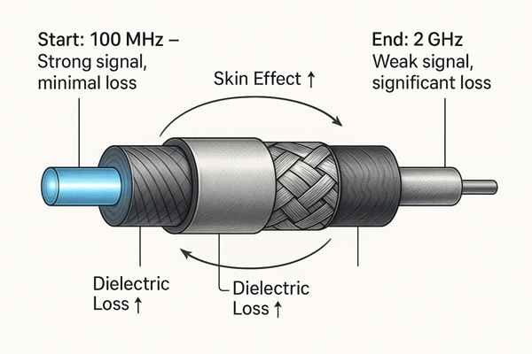
Frequency-dependent signal loss in coaxial cables is caused by two main factors: the skin effect and dielectric loss. The skin effect increases conductor resistance at higher frequencies, while dielectric loss involves the absorption of RF energy by the insulating material. Both losses worsen as frequency increases.

This table summarizes the two main loss mechanisms:

Feature	Skin Effect4	Dielectric Loss5
Primary Cause	Current crowding on conductor surface	Energy absorbed by the insulator material
Proportionality	Proportional to \(\sqrt{f}\)	Proportional to \(f\)
Dominant Range	Lower frequencies (\(< 1 \text{ GHz}\))	Higher frequencies (\(> 1 \text{ GHz}\))
Mitigation	Larger conductor diameter, silver plating	Low-loss dielectrics (PTFE, Foamed PE)

For copper, the skin depth is about \(6.6 \text{ }\mu\text{m}\) at 100 MHz but shrinks to just \(1.3 \text{ }\mu\text{m}\) at 2.4 GHz. Dielectric loss is related to a material's loss tangent, \(\tan\delta\).

---

What is the Cutoff Frequency of a Coaxial Cable?

You've selected a cable rated for high frequencies, yet you're seeing strange signal behavior. Pushing a cable beyond its intended operating mode can introduce unexpected distortion and system failure.

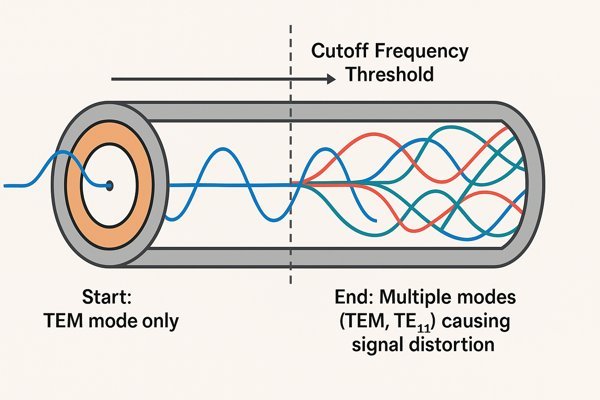
The cutoff frequency is the point where a coaxial cable starts supporting electromagnetic modes other than its primary TEM mode. This first higher-order mode is typically the \(TE_{11}\) mode. Operating above this frequency causes signal degradation because multiple modes travel at different speeds, distorting the signal.

The cutoff frequency (\(f_{c}\)) is determined by the cable's physical dimensions and dielectric material.

The Governing Formula

As defined in standards like MIL-HDBK-216, the cutoff frequency⁶ is approximately:
\(f_{c} \approx \frac{c}{\pi \frac{d+D}{2} \sqrt{\epsilon_{r}}}\)
Where \(d\) is the inner conductor's diameter, \(D\) is the shield's inner diameter, and \(\epsilon_{r}\) is the dielectric constant⁷.

Cutoff Frequency Examples

This table shows how small changes in dimensions can dramatically affect the theoretical limit. For a typical RG58 cable⁸ with \(\epsilon_{r} \approx 2.25\), \(d = 0.9 \text{ mm}\), and \(D = 2.95 \text{ mm}\), the cutoff frequency is \(\approx 19 \text{ GHz}\).

Cable Type	Inner Diameter (\(d\))	Outer Diameter (\(D\))	Dielectric (\(\epsilon_{r}\))	Approx. Cutoff Freq. (\(f_{c}\))
RG58/U	\(0.9 \text{ mm}\)	\(2.95 \text{ mm}\)	2.25 (PE)	\(\approx 19 \text{ GHz}\)
RG174	\(0.48 \text{ mm}\)	\(1.5 \text{ mm}\)	2.25 (PE)	\(\approx 44 \text{ GHz}\)
RG316	\(0.51 \text{ mm}\)	\(1.52 \text{ mm}\)	2.1 (PTFE)	\(\approx 46 \text{ GHz}\)

Important Note: The practical operating frequency is always much lower than the cutoff frequency due to excessive attenuation.

---

What is the Transverse Electromagnetic (TEM) Propagation Mode?

We talk about signals traveling through cables, but what does that really mean? Not understanding the fundamental mode of propagation can lead to poor design choices and unexpected issues.

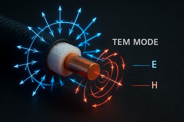
The Transverse Electromagnetic (TEM) mode is the primary way signals travel in a coaxial cable. In TEM mode, both the electric (\(E\)) and magnetic (\(H\)) fields are perpendicular (transverse) to the direction of signal travel. This mode is ideal because it has no lower cutoff frequency.

Visualizing the Electric and Magnetic Fields

Imagine looking at a cross-section of a coaxial cable. In TEM mode, the electric (\(E\)) field lines radiate straight out from the center conductor to the shield. The magnetic (\(H\)) field lines form perfect circles around the center conductor. Both of these fields are at a 90-degree angle to the direction the signal is moving down the cable.

Why TEM Mode is Ideal

This clean, predictable field structure is what allows a coaxial cable to transmit signals from DC all the way up to its cutoff frequency. Other waveguides, like a hollow metal pipe, cannot support TEM mode and have a non-zero lower frequency limit. The beauty of TEM mode is its simplicity and broad bandwidth, ensuring all frequency components of a complex signal travel at the same speed, thus preserving the signal's shape.

---

What are the Key Differences Between Common 50Ω RF Coaxial Cables?

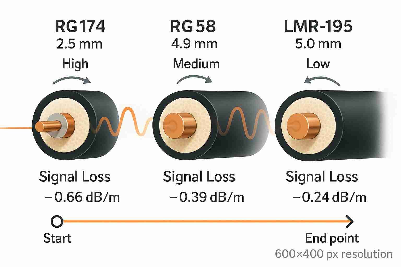
Choosing between RG58, RG174, and LMR-195 feels like a guessing game. Selecting the wrong one can mean excessive signal loss or unnecessary cost and bulk in your design.

The main differences between common \(50 \Omega\) RF coaxial cables are their physical size, attenuation characteristics, and maximum frequency. For example, RG174 is thin and flexible but has high loss. RG58 is a general-purpose standard, while LMR-195 offers significantly lower loss and better shielding for high-performance applications.

As an engineer, choosing the right cable is about balancing trade-offs between performance, cost, and physical constraints.

Comparative Analysis

Here’s a practical breakdown:

Feature	RG174	RG58/U	LMR-195-UF
Attenuation @ 1 GHz	\(\approx 44 \text{ dB} / 100 \text{ ft}\)	\(\approx 19 \text{ dB} / 100 \text{ ft}\)	\(\approx 10.7 \text{ dB} / 100 \text{ ft}\)
Use Case	Short jumpers, GPS antennas	General lab use, (\(<1 \text{ GHz}\))	High-performance Wi-Fi/cellular links

---

Why is Maintaining a Cable's Characteristic Impedance Critical in High-Frequency Circuits?

Are signal reflections and poor VSWR plaguing your RF system? These issues often point back to one critical parameter that has been overlooked: characteristic impedance.

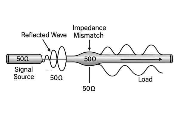
Maintaining a constant \(50 \Omega\) or \(75 \Omega\) characteristic impedance is critical because any change creates a mismatch. This mismatch causes signal reflections, where part of the signal bounces back toward the source. This leads to signal loss (VSWR), ringing, and distortion, severely degrading system performance.

The Physics of Reflection and VSWR

Characteristic impedance (\(Z_{0}\)) is a property determined by the cable's physical construction. For a \(50 \Omega\) system, every component must present a \(50 \Omega\) impedance. When the signal encounters a point where the impedance changes, a portion of its energy is reflected. This is quantified by the Voltage Standing Wave Ratio (VSWR)⁹. A perfect match has a VSWR of 1:1. A VSWR of 2.0:1 means over 11% of the power is reflected.

A Debugging War Story

This reflected power not only fails to reach the destination but can damage components. I once spent a week debugging a Wi-Fi module that kept failing certification. The issue wasn't the chip; it was a poorly specified pigtail cable whose impedance varied along its length, creating significant reflections and failing our spurious emissions tests.

---

How do Coaxial Connectors Impact the Frequency Limit of a Cable Assembly?

You've carefully selected a high-frequency cable, but did you consider the connectors? The wrong connector can act as a bottleneck, completely negating the performance of your expensive cable.

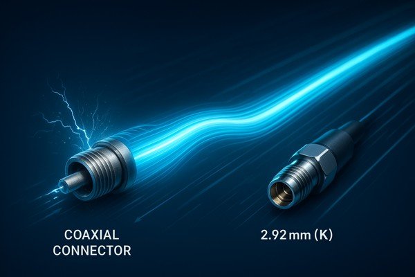
Coaxial connectors are a primary limiting factor for an assembly's frequency performance. Each connector type has a maximum usable frequency determined by its physical size and geometry. For example, a standard SMA connector is typically rated up to 18 GHz, while a precision 2.92mm (K) connector works up to 40 GHz.

Frequency Ratings for Common Connectors

As frequency increases, the connector's physical size becomes a significant fraction of the signal's wavelength, which is why smaller connectors generally have higher frequency ratings.

Connector Type	Typical Max Frequency
BNC	4 GHz
N-Type	11 GHz
SMA	18 GHz
3.5mm	34 GHz
2.92mm (K)	40 GHz
1.85mm (V)	67 GHz

---

How are S-Parameters Used to Characterize a Coaxial Cable's Performance?

Your datasheet provides basic loss figures, but how does your cable assembly really perform across a frequency band? Without S-parameters, you're flying blind when it comes to high-frequency characterization.

S-parameters (Scattering parameters) precisely characterize a coaxial cable's performance. The two most important are \(S_{21}\) (Insertion Loss), which measures how much signal gets through the cable, and \(S_{11}\) (Return Loss), which measures how much signal is reflected back due to impedance mismatches.

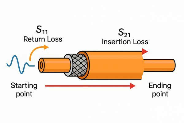
"Coaxial Cable Signal Reflection and Transmission Loss")

When I debugged the PACE evaluation board for Lightelligence, we relied heavily on a Vector Network Analyzer (VNA) to measure S-parameters. This was critical for verifying every high-speed path.

Key S-Parameters Explained

This table clarifies the most important S-parameters for a cable assembly.

Parameter	Name	What It Measures	Ideal Value (for a cable)
\(S_{11}\)	Return Loss10	Signal reflected back at the input	As low as possible (\(< -15 \text{ dB}\))
\(S_{21}\)	Insertion Loss11	Signal that passes through from input to output	As close to 0 dB as possible
\(S_{12}\)	Reverse Isolation	Signal passing from output to input	Same as \(S_{21}\) for a passive cable
\(S_{22}\)	Output Return Loss	Signal reflected back at the output	Same as \(S_{11}\) for a symmetric cable

---

How Does a Coaxial Cable's Bandwidth Affect the Integrity of High-Speed Digital Signals?

Are you seeing closed eye diagrams and bit errors in your high-speed digital interface? The problem might not be your driver or receiver, but the analog limitations of your coaxial cable.

A coaxial cable's bandwidth directly impacts high-speed digital signal integrity. A cable with insufficient bandwidth acts as a low-pass filter, slowing down the signal's rise and fall times. This causes inter-symbol interference (ISI) and a "closed" eye diagram, leading to increased bit error rates.

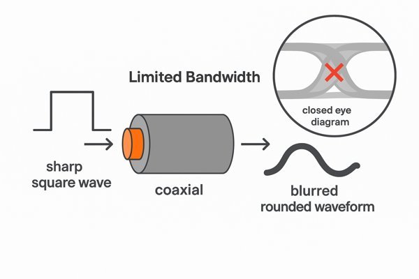
The Birth of Inter-Symbol Interference (ISI)¹²

A sharp digital pulse is composed of a fundamental frequency and a wide spectrum of higher-frequency harmonics. A common rule of thumb is that the cable's bandwidth needs to be at least half of the signal's bit rate. For a 10 Gbps signal, you need a cable with good performance up to at least 5 GHz. When a cable filters out the crucial high-frequency harmonics, it rounds off the sharp edges of the pulses. This causes the end of one bit to smear into the beginning of the next, a phenomenon called Inter-Symbol Interference (ISI).

Visualizing the Problem: The Eye Diagram

When visualized on an oscilloscope using an eye diagram, this ISI effect shrinks the opening of the "eye." A smaller eye opening leaves less margin for noise and timing jitter, directly leading to a higher Bit Error Rate (BER)¹³.

---

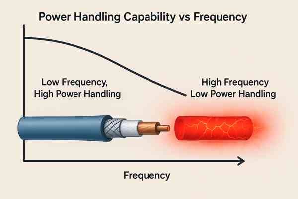
How Does Operating Frequency Affect a Coaxial Cable's Power Handling Capability?

Have you ever experienced a cable failure when pushing high power at high frequencies? It's a costly and dangerous problem caused by overlooking a critical cable limitation.

A coaxial cable's power handling capability decreases significantly as the operating frequency increases. This is because both conductor and dielectric losses generate more heat at higher frequencies. This heat can damage the dielectric insulator, leading to a catastrophic failure of the cable.

The Limiting Factor: Dielectric Temperature

A cable's power rating is limited by the maximum temperature its dielectric can withstand. For standard PE, this is around \(85^{\circ}\text{C}\), while for PTFE it's over \(200^{\circ}\text{C}\).

Power vs. Frequency Example (LMR-400)

All signal loss is converted into heat. Since losses increase with frequency, the power a cable can safely handle drops dramatically, as shown in this table for LMR-400.

Frequency	Average Power Handling*
100 MHz	\(1100 \text{ W}\)
900 MHz	\(330 \text{ W}\)
2.4 GHz	\(180 \text{ W}\)
5.8 GHz	\(110 \text{ W}\)

*Note: Based on \(40^{\circ}\text{C}\) ambient temperature, sea level.

---

What are the Advantages of Using Microstrip Over Coaxial Cables for Board-Level RF Transmission?

Running tiny coaxial cables across a crowded PCB is a manufacturing nightmare. There has to be a better way to route RF signals directly on the board without sacrificing performance.

For board-level RF, microstrip transmission lines offer significant advantages over coaxial cables. They are cheaper to fabricate as they are integrated directly into the PCB layout. This also simplifies assembly and allows for easier integration with surface-mount components, reducing complexity and cost for mass production.

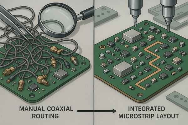
While coaxial cables offer excellent shielding, they are impractical for routing signals between chips on a single PCB. This is where planar transmission lines like microstrip come in.

Microstrip vs. Coaxial Cable

This table provides a high-level comparison for board-level interconnects.

Feature	Microstrip Transmission Line	Coaxial Cable Assembly
Shielding	Lower	Higher
Integration	Excellent (part of PCB)	Poor (separate component)
Assembly	Simple (etched with PCB)	Complex (requires connectors, mounting)
Cost	Very Low	High
Noise Immunity	Lower	Higher
Typical Loss	Higher for a given length	Lower for a given length

However, for most board-level interconnects at frequencies \(< 20 \text{ GHz}\), the benefits of integration and cost far outweigh these drawbacks.

---

Conclusion

A coaxial cable's frequency limit is not one number but a balance of attenuation, cutoff frequency, and component choice. Mastering RF design means understanding these trade-offs to deliver a reliable, high-performance product.

---