Skip to content
Struggling with signal integrity issues like ringing and reflections? Your PCB traces might be acting as antennas, causing unpredictable behavior and project delays.
A trace must be treated as a transmission line when its length is a significant fraction of the signal's electrical wavelength. The most common rule is to apply transmission line design principles when the trace's round-trip delay is longer than the signal's fastest rise or fall time.

Understanding this rule is the first step, but a lot more goes into making sure your high-speed signals arrive clean and on time. These effects can make or break a design, especially as clock speeds and data rates continue to climb. Let's break down exactly what these effects are, when you need to worry about them, and how to manage them in your designs to ensure your product works reliably.
What Is the Transmission Line Effect?
Ever sent a perfect square wave down a trace only to see a garbled mess at the other end? That is the transmission line effect in action.
The transmission line effect describes how a physical conductor, like a PCB trace, behaves when carrying high-frequency signals. It stops being a simple wire. Its distributed inductance and capacitance create a characteristic impedance, causing reflections, ringing, and delays if not properly managed.

How a Simple Wire Becomes a Complex System
At DC or very low frequencies, a PCB trace acts like a simple resistor. The signal is the same at all points along the trace at any given instant. But as signal speeds increase, this simple model breaks down. The trace must be viewed as a complex system with distributed components.
From Simple Wire to Distributed System
A high-speed signal's changing electric field creates capacitance (\(C\)) between the trace and its reference plane (usually a ground plane). At the same time, the changing current creates a magnetic field, which results in series inductance (\(L\)). These are not single "lumped" components but are distributed continuously along the entire length of the trace. This is often visualized with the RLCG model1, where each tiny segment of the trace has series resistance (\(R\)), series inductance (\(L\)), shunt capacitance (\(C\)), and shunt conductance (\(G\)) to the reference plane.
The Origin of Reflections
This structure of distributed \(L\) and \(C\) creates what we call characteristic impedance2 (\(Z_{0}\)), which is approximately \(\sqrt{L/C}\). This is an intrinsic property of the trace geometry and PCB materials. When a signal travels down this trace, it expects to see this impedance continuously. If the signal reaches the end of the line and the load's impedance (\(Z_{L}\)) doesn't perfectly match \(Z_{0}\), the energy cannot be fully absorbed. A portion of the signal energy reflects back toward the source, much like how an ocean wave reflects off a seawall. The amount of reflection is determined by the reflection coefficient, Gamma3 (\(\Gamma\)), calculated as: \(\Gamma = \frac{Z_{L} - Z_{0}}{Z_{L} + Z_{0}}\). A perfect match means \(Z_{L} = Z_{0}\), so \(\Gamma = 0\) and there is no reflection. A large mismatch results in a large reflection, which interferes with the original signal and causes the ringing and overshoot that corrupts your data.
When to Treat a Trace as a Transmission Line?
Unsure if that 5cm trace needs special attention? Guessing can lead to costly board respins and frustrating debugging sessions when your circuit fails unexpectedly.
You must treat a trace as a transmission line when it is "electrically long." A trace is considered electrically long if its length allows the signal to change significantly while it is propagating down the trace. The standard engineering rule is when the trace length is longer than the distance a signal travels during half of its rise time.

Calculating the Critical Trace Length
The decision to use transmission line techniques depends on comparing the signal's speed to the trace's physical length. A fast signal edge contains high-frequency content, regardless of the clock's frequency. This is why we focus on the signal's rise time (\(t_{r}\)) or fall time (\(t_{f}\))4. You can typically find this crucial value in the component's datasheet under "Electrical Characteristics" or, for more detail, within its IBIS model.
The Critical Length Rule
A trace becomes a transmission line when its one-way propagation delay (\(T_{pd}\))5 is a significant fraction of the signal's rise time. The "critical length" (\(L_{\text{critical}}\)) can be calculated. A common formula used is:
\(L_{\text{critical}} = \frac{t_{r}}{2 \times T_{pd\_\text{per}\_\text{length}}}\)
Critical Length for Common Interfaces
Let's apply this to some common standards, assuming a typical FR-4 propagation delay of 160 ps/inch (\(\approx\)63 ps/cm):
| Interface | Typical Rise Time (\(t_{r}\)) | Critical Length (Approx.) | Action |
|---|---|---|---|
| I2C (400 kHz) | 100 ns | \(\approx\)800 cm | Ignore transmission line effects |
| USB 2.0 (480 Mbps) | 500 ps | \(\approx\)4 cm (1.6 inches) | Must use 90 \(\Omega\) controlled impedance |
| DDR3 (1600 MT/s) | 150 ps | \(\approx\)1.2 cm (0.47 inches) | Must use 100 \(\Omega\) diff / 50 \(\Omega\) SE |
| PCIe 3.0 (8 GT/s) | 40 ps | \(\approx\)0.3 cm (0.12 inches) | Must use 85/100 \(\Omega\), critical layout |
As you can see, for any modern high-speed interface, almost every trace is electrically long and requires careful transmission line design.
When Can Transmission Line Effects Be Ignored?
Worried about over-engineering your simple boards? Wasting time and money on unnecessary impedance control for every single trace is a common and costly mistake.
You can safely ignore transmission line effects when the trace is "electrically short." This means its physical length is much shorter than the critical length. In this case, reflections return to the source so quickly that they don't have time to interfere with the rising edge of the signal.

Understanding "Electrically Short" Traces
When a trace is electrically short, the signal's voltage is essentially the same at every point along the trace at any given moment. This allows us to use a simpler "lumped element" model instead of the complex "distributed element" model of a transmission line.
The Lumped Element Model6
For an electrically short trace, we can approximate its total parasitic inductance and capacitance as single, discrete components. The trace acts more like a simple R-C or R-L-C low-pass filter. While these parasitics can still cause issues like slowing down the signal's edge rate, they won't cause the destructive ringing and reflections characteristic of a mismatched transmission line. This simplifies the design process significantly because you don't need to worry about precise impedance matching.
An Example with a Slow Signal
Consider a slow SPI signal running at 1 MHz. The rise time is often in the range of 50-100 ns. Let's be conservative and use \(t_{r} = 50 \text{ ns}\). Using the same FR-4 material from before (\(T_{pd} \approx 63 \text{ ps/cm}\)):
\(L_{\text{critical}} = \frac{50 \text{ ns}}{2 \times 63 \text{ ps/cm}} = \frac{50,000 \text{ ps}}{126 \text{ ps/cm}} \approx 396 \text{ cm}\) (or nearly 4 meters).
It's impossible to have a 4-meter SPI trace on a single PCB. In this scenario, even a long 15 cm trace is electrically short. You can ignore transmission line effects and focus only on ensuring the total capacitive load is within spec and that the signal has sharp enough edges for the receiver. This is why you don't see impedance control requirements for low-speed interfaces.
What Are the Key Considerations for Transmission Line Design?
So you know you need a transmission line, but what now? Incorrectly implementing one is just as bad as ignoring the effect in the first place.
The three key considerations are: 1) defining the Characteristic Impedance (\(Z_{0}\)) required by the interface, 2) controlling Trace Geometry and PCB Stack-up to achieve that impedance, and 3) implementing a proper Termination scheme to prevent reflections.

Implementing a Successful Transmission Line
Successful transmission line design is a collaboration between you and your PCB fabricator. It requires careful planning before you even start routing traces.
1. Characteristic Impedance (\(Z_{0}\)) and Stack-up
The target impedance is usually defined by the technology standard (e.g., 50 \(\Omega\) single-ended, 100 \(\Omega\) differential for DDR4). To achieve this impedance, you must control the physical dimensions of the trace and its environment. The main factors are:
- Trace Width (\(W\))
- Dielectric Height (\(H\)): The distance from the trace to its reference plane.
- Dielectric Constant (\(\epsilon_{r}\)): A property of the PCB material.
You must provide your impedance requirements to your PCB fab house. They will then propose a stack-up that defines the layer thicknesses and corresponding trace widths to hit your target \(Z_{0}\).
2. Termination Schemes
Termination is the act of adding a resistor to the line to match the load impedance to the trace's characteristic impedance. This ensures that when the signal arrives, its energy is absorbed rather than reflected. Common methods include:
| Termination Scheme | Location | Key Characteristic | Best Use Case |
|---|---|---|---|
| Series | At the source, near the driver. | Simple, no static power draw. | Point-to-point connections. |
| Parallel | At the load, to VCC or GND. | Excellent signal quality, but consumes static power. | High-speed buses, end of the line. |
| Thevenin | At the load, voltage divider. | Very effective termination, but highest power draw. | Noisy environments where signal level is critical. |
| AC | At the load, R and C in series. | No DC power draw, blocks DC bias. | AC-coupled signals (e.g., SATA, PCIe). |
3. Routing Best Practices
- Continuous Reference Plane: The trace must always have a solid, unbroken ground or power plane directly adjacent to it. Routing over a split in this plane is the #1 cause of signal integrity and EMI failure.
- Differential Pairs: Route the P and N traces as a tightly coupled pair. Keep their lengths matched to within a very tight tolerance (e.g., \(< 5 \text{ mils}\) for PCIe) to prevent common-mode noise.
- Vias: Vias introduce an impedance discontinuity. For very high-speed signals, every via matters. Use "stitching vias" near your signal via to provide a short return current path between ground planes.
- Length Matching: For parallel buses like DDR, all data and strobe lines must be length-matched to ensure signals arrive at the same time. This is often done using serpentine routing to add length to shorter traces.
What Is the Condition for a Transmission Line to Be Considered Lossless?
You often hear engineers talk about "lossless" lines and might wonder if it's even possible. Understanding this ideal concept helps you manage real-world, lossy lines better.
A transmission line is considered theoretically lossless when its series resistance (\(R\)) and its shunt conductance (\(G\)) are both exactly zero. In this ideal physical model, a signal can propagate along the line without any loss of energy or amplitude.

The Theory Behind a Lossless Line
The full RLCG model of a transmission line accounts for all physical effects. By setting certain parts of this model to zero, we can create a useful simplification that makes analysis much easier.
The RLCG Model Simplified
The full model for a tiny segment of a transmission line includes four elements:
- \(R\) (Series Resistance): Represents the energy lost as heat in the conductor (e.g., copper trace).
- \(L\) (Series Inductance): Represents the energy stored in the magnetic field around the conductor.
- \(C\) (Shunt Capacitance): Represents the energy stored in the electric field between the conductor and its reference plane.
- \(G\) (Shunt Conductance): Represents the energy lost as heat in the dielectric material separating the conductor and reference plane.
The Idealization
To create the lossless model, we assume we are using a perfect conductor (superconductor) so that \(R = 0\), and a perfect insulator (a vacuum) for the dielectric so that \(G = 0\). This leaves only the ideal energy storage elements, \(L\) and \(C\). In this case, the math simplifies greatly. The characteristic impedance, \(Z_{0} = \sqrt{(R+j\omega L)/(G+j\omega C)}\), becomes purely real and frequency-independent: \(Z_{0} = \sqrt{L/C}\). The signal's amplitude remains constant as it travels, though its phase still changes. This model is a useful fiction. It allows us to calculate impedance and reflections without getting bogged down in the complex math of losses.
What Is the Difference Between a Lossless and a Low Loss Transmission Line?
Your material datasheet says "low loss," but your simulation software has a "lossless" option. Are they the same thing? Knowing the difference is key to accurate high-frequency design.
A lossless line is a theoretical ideal where resistance (\(R\)) and conductance (\(G\)) are zero. A low-loss line is a practical, real-world line where \(R\) and \(G\) are very small but not zero. Low-loss lines still cause some signal attenuation (loss of amplitude), especially at high frequencies.

From Theory to Real-World Materials
In the real world, no transmission line is perfect. The distinction between "low loss" and "standard loss" is critical for high-performance applications.
Real-World Loss Mechanisms
There are two primary sources of loss in a PCB trace. The table below outlines these loss types and when they become a major concern.
| Loss Type | Physical Cause | Dominant Factor | When It Becomes Critical |
|---|---|---|---|
| Dielectric Loss7 | Energy absorbed by the PCB's insulating material. | Material's Loss Tangent (\(\tan\delta\)). | Frequencies \(>5 \text{ GHz}\). Becomes the primary loss factor at very high frequencies. |
| Conductor Loss | Resistive heating of the copper trace. | Skin effect and copper surface roughness. | Across all high frequencies, but especially significant where traces are long and thin. |
Choosing the right material is a cost-performance trade-off. For my work on photonic computing chips with 28 Gbps+ signals, standard FR-4 was not an option; low-loss laminates with smooth copper were essential for the system to function at all.
In Which Among the Transmission Lines Can the Capacitance Effect Be Neglected?
Can you ever just ignore capacitance? It's a fundamental part of every circuit, and misunderstanding its role in transmission lines can lead to complete design failure.
The capacitance effect can never be truly neglected in a standard transmission line like a microstrip or stripline. The distributed capacitance (\(C\)) and inductance (\(L\)) are the two fundamental properties that define the line's characteristic impedance (\(Z_{0} \approx \sqrt{L/C}\)).

Why Capacitance Is Not Optional
This question touches on the very definition of a transmission line. To ask when capacitance can be ignored is to fundamentally misunderstand what a transmission line is.
The Core L-C Definition
A transmission line works by propagating an electromagnetic wave along a structure. This wave consists of both an electric field (related to capacitance) and a magnetic field (related to inductance). They are inseparable. Removing the capacitance from the model would mean \(Z_{0}\) becomes infinite, which is physically meaningless. It's like asking when the wheels on a car can be neglected; they are part of its basic definition.
Misinterpreting the Question
Perhaps the question is intended to ask when capacitance is not the dominant effect. For example, if you have an extremely short trace, you are no longer in the transmission line domain but in the "lumped element" domain. In this case, you might find that the trace's total resistance has a greater impact on the circuit than its total capacitance. But once a trace is long enough to be considered a transmission line, both \(L\) and \(C\) are, by definition, critically important.
A Special Case: Waveguides
The only transmission structure where the L-C model isn't used directly is a hollow metallic waveguide, which is typically used for extremely high microwave or millimeter-wave frequencies (\(>20 \text{ GHz}\)). In a waveguide, the EM wave propagates inside a hollow tube. We analyze this using Maxwell's field equations and "modes" (TE/TM modes) rather than a simple circuit model. However, even here, electric and magnetic fields are absolutely essential for the wave to exist. So even in this exotic case, the underlying physical principles related to capacitance and inductance are still at play.
What Is the Smith Chart in Transmission Line?
That strange, circular chart looks intimidating, doesn't it? But failing to learn it means you are just guessing when it comes to high-frequency impedance matching.
The Smith Chart is a graphical calculator used by RF and high-frequency engineers to solve transmission line problems. It cleverly maps the complex impedance plane onto a circle, turning difficult complex number calculations into simple geometric movements on the chart.

Using the Smith Chart8 for Impedance Matching9
The Smith Chart is one of the most powerful tools in an RF engineer's toolkit. It was revolutionary when it was invented because it replaced pages of tedious math with a simple graphical process.
How It Works
The chart turns complex math into simple geometry.
- The center of the chart represents the system's characteristic impedance (e.g., a perfect 50 \(\Omega\) match).
- Moving along a circle of constant radius on the chart is equivalent to moving physically along the transmission line.
- Adding components corresponds to moving along specific arcs. Adding a series component (\(L\) or \(C\)) moves the point along a constant resistance circle. Adding a parallel (shunt) component moves the point along a constant conductance circle.
Practical Use: Impedance Matching
Let's say I have a Wi-Fi antenna with an impedance of \(30 - j25 \Omega\) at 2.4 GHz, and I need to match it to my 50 \(\Omega\) system.
- I would first plot the normalized impedance point on the chart.
- My goal is to add components to move this point to the center of the chart (the perfect match).
- By following the circles and arcs, I can graphically determine that adding, for example, a series inductor of a specific value and then a parallel capacitor of another specific value will land me exactly at the center. This is far faster and more intuitive than solving the equations by hand. I used this technique extensively at Honeywell when designing and tuning Wi-fi matching networks for optimal performance.
How Do You Know If Your Transmission Line Is Bad?
Your board is built, but the system is flaky and unreliable. Is it a software bug, a bad chip, or is your PCB layout to blame for the problems?
You know your transmission line is bad if you see symptoms like signal ringing, significant overshoot/undershoot, a closed eye diagram on an oscilloscope, or if your device fails electromagnetic interference (EMI) testing. These are all direct results of impedance mismatches and reflections.

Diagnosing a Faulty Transmission Line
A "bad" transmission line is one that doesn't deliver a clean, predictable signal to the receiver. The problems it creates can be subtle and hard to diagnose, often appearing as intermittent system failures. The table below summarizes the key diagnostic methods.
| Diagnostic Method | Tools Needed | What It Reveals |
|---|---|---|
| Visual Inspection | High-bandwidth oscilloscope, probes. | Signal quality issues like overshoot, ringing, and slow rise times. A closed eye diagram indicates a high bit error rate. |
| Advanced Diagnosis | Time-Domain Reflectometer (TDR)10. | A complete impedance profile of the trace. Pinpoints the exact physical location of faults like opens, shorts, or bad vias. |
| Functional & EMI Testing | System-level tests, EMC test chamber. | Intermittent system failures, data corruption, or failure to meet regulatory EMI standards (FCC, CE). |
1. Visual Inspection with an Oscilloscope
Probing the signal at the receiver IC pin will reveal the truth.
- Overshoot & Ringing: The signal voltage flies past its target voltage (e.g., 3.3V) and then oscillates. Severe overshoot can damage input pins on ICs, while ringing can cause false clock edges, leading to data corruption.
- Closed Eye Diagram: For high-speed serial links (like SATA or PCIe), we use an eye diagram. A good transmission line results in a wide-open "eye." A bad, lossy, or mismatched line will cause the eye to close, indicating a high probability of bit errors.
2. Advanced Diagnosis with a TDR
For professional-grade debugging, the ultimate tool is a Time-Domain Reflectometer (TDR). A TDR works like radar for your PCB. It sends a very fast pulse down the trace and listens for reflections. The output is a graph of impedance versus distance along the trace. This allows you to verify the characteristic impedance of your trace and pinpoint the exact physical location of a fault.
3. Functional and EMI Failures
- Functional Failures: The device works intermittently, fails at higher temperatures, or corrupts data. These are classic signs that signal integrity is marginal.
- EMI/EMC Failures: A poorly designed transmission line acts as an efficient antenna. It radiates high-frequency energy that will cause your product to fail regulatory compliance tests, forcing a costly board respin.
Conclusion
Mastering transmission line theory is no longer optional for hardware engineers. Treating electrically long traces with care by controlling impedance and using proper termination is essential for creating reliable, high-performance products.
-
Understanding the RLCG model is crucial for grasping how PCB traces behave at high frequencies, impacting signal integrity. ↩
-
Exploring characteristic impedance helps in designing circuits that minimize signal reflections and improve performance. ↩
-
Learning about the reflection coefficient Gamma is essential for understanding signal integrity and minimizing data corruption. ↩
-
Understanding rise and fall times is crucial for designing high-speed circuits, as they directly impact signal integrity and transmission line effects. ↩
-
Understanding propagation delay is essential for designing high-speed circuits, as it directly impacts signal integrity and trace length decisions. ↩
-
Understanding the Lumped Element Model is crucial for simplifying circuit design and analyzing electrical components effectively. ↩
-
Understanding Dielectric Loss is crucial for optimizing PCB performance, especially in high-frequency applications. ↩
-
Explore this link to understand the Smith Chart's significance in RF engineering and its practical applications. ↩
-
Learn about impedance matching techniques to enhance your understanding of RF circuit design and performance. ↩
-
Understanding TDR can enhance your debugging skills, helping you locate faults in transmission lines effectively. ↩